Variable rate applications based on your soil
by Marnus Ferreira, Head of Soil Science
Yield data still a popular choice
The application of variable rate soil corrections such as lime and gypsum is not new to the agricultural industry while the benefits in terms of cost savings and soil fertility flowing from these applications are well known. Despite this, many producers are still far from making adequate use of variable rate systems during fertilisation and planting (or sowing), while in fact far greater benefits could be achieved by doing so.
There are various reasons for an apparent reluctance to embrace these systems, which, to some extent, are understandable. Firstly, the technology is challenging and relatively unknown. Then there seems to be a resistance to change and a mindset that what has been done throughout the years up to now has worked sufficiently, resulting in change taking place very slowly. The biggest reason, however, is the uncertainty surrounding the type of information or data on which variable rate maps should be based. In this regard many producers consider the use of harvest or yield data to be the easiest. However, the question must be asked whether this method still provides sufficient results.
The risk
What is often witnessed in practice is that a well performing field performs progressively worse over time due to lack of adequate fertility, acid saturation, compaction etc. Year-on-year planting on the field is reduced, resulting in a reduction in yield, all because the underlying problem is never addressed. The use of yield data alone therefore carries great risk. It is for this reason that the most precious and durable asset should rather be looked at for answers, namely the soil.
The answers lie in the soil
This statement has been motivated by results achieved in a long term “trial” Agri Technovation (AT) was and still is involved in.
The trial
A portion of a crop farm (± 500 ha) and about a third of the total planted surface area is used to make decisions, which are then applied to the rest of the farm. A practice, cultivar, implement or machine is applied to or used on the 500 ha experimental farm and, if successful, transferred to the rest of the farm.
Results achieved were based on 7 years of data on variable rate applications of potassium (combination of KCl and cattle manure), lime (calcitic and dolomitic, as needed), gypsum, phosphate (combination of MAP and cattle manure), as well as 5 years of complete harvest data. It must be emphasised that the practices that resulted in real success were based on accurate, scientifically-determined data. Therefore, the exact measurement as well as the correct use/application of the correct tool/practice are both required for the trial to be successful and the producer to truly reap the benefits. Without one or the other, it will not work.
Data collection
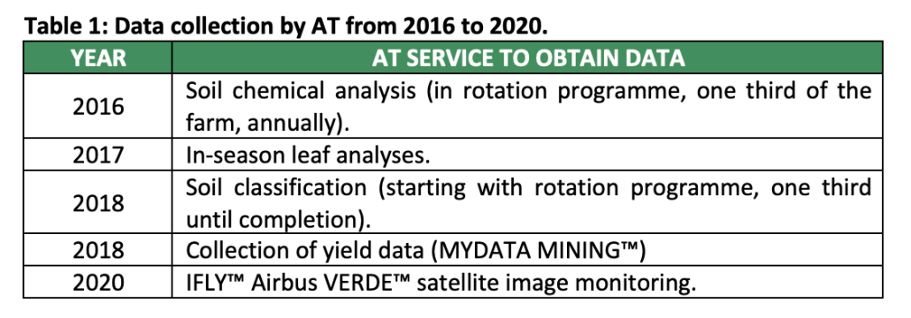
The data collection component for the trial included the following AT services provided over the time periods indicated (Table 1).
Corrections
Variable rate soil corrections were applied from 2016.
Data processing
In 2019, AT processed the yield data and linked it to all the respective datasets obtained (Table 1), to determine correlations and draw comparisons around crop and cultivar preferences. These correlations and comparisons are based on thousands of actual data points. The data derived significantly strengthened the value of the information in terms of which decisions were made.
Impact on soil fertility
Improved soil fertility and reduced costs
The real (actual) impact on soil fertility is outlined below with reference to a few examples (Figures 1, 2 and 3). The results clearly indicate that the variable rate applications of soil corrections altered soil fertility in such a way that significantly fewer corrections are currently required, resulting in reduced costs to the producer.
Maintaining a good soil fertility status with variable rate applications is much easier than starting the process of correcting the soil, but the fruits of the labour will eventually be reaped. The impact over time is typically as shown in Table 2 (and as was found in the trial): Fewer hectares need to be corrected and less product is required (applied) to maintain a good soil fertility status.

Example 1
Figure 1. Potassium (K) in ppm or parts per million for 2016 (left) and 2022 (right). The variable correction maps (in purple) for 2016 (left) and 2022 (right) (for MAP) are indicated. Note the distinct change in overall soil fertility from 2016 to 2022, as well as the significantly smaller surface area that needs corrections.

Table 2: The total hectares, tonnes and average kg/ha KCl applied for the periods 2016 and 2022. Note the remarkable change over time of quantities required to maintain good soil fertility.
Example 2
The graph (Figure 2) shows the difference in yield between the experimental farm and the rest of the farm. (Experimental farm indicated in green.) The yield consistency on the experimental farm, even during the challenging years, is noteworthy: an average of 8.8 t/ha over a 5-year period. The rest of the farm produced a 5-year average of 7,92 t/ha.
Over a period of 5 years, this is a difference of 880 kg/ha. Also, the positive impact of the practices is not as distinctly noticeable for the better performing years, but clearly more noticeable for the challenging years.
This however, is only one part to the story. One can, of course, “buy” yields that could result in short term success, but long-term success is achieved by farming profitably. This brings us to the last graph (Figure 3).
Example 3
Figure 3 indicates the profitability of the two respective areas.
Break-even (the red line) is 1, and represents the imaginary one (1) rand that is required to plant. Performance below the break-even-R1 line means there is a loss. For example, if the figure is 0,95 it means that 5 cents to every R1 invested is effectively paid in. Certainly not an ideal investment.
To achieve effective growth, a producer would naturally want the farm to perform in the positive category (well above the red line), typically above RSA’s current inflation figure. This is the precise principle upon which long-term successful farming is based.
It is of course possible to do a hypothetical calculation around “flat rate” K corrections based on extraction, but that sum total will reflect badly on the precision correction, because in this case, the original K correction was very costly – the soils were in very poor condition due to the application of “conventional” practices. The corrections calculation therefore makes a lot more sense over time. We did however want to highlight this as it represents the correct figures and focusses on the total input vs output (includes everything: diesel, seed, harvest insurance etc.).
Thus, although the first corrections were expensive, it was a once-off expense, and resulted in the profitability of the farm being significantly higher from 2018 – 2021 than that of the rest of the farm.
This article focuses on an actual case study on the greater impact of a 500 ha farm within a 1500+ ha farm, that is farmed 100% on a precision approach. The success story of a precision approach is directly compared to a flat-rate approach on a large-scale level.
The other fields are also measured by way of precision sampling, but corrections were not necessarily made with precision equipment, while this was indeed the case on the “experimental farm”. We therefore did not want to ask a hypothetical question, but rather show the actual figures. A focus on the hypothetical difference will require the writing of a completely different article (which will also have a lot of value).
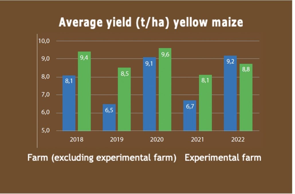
Figure 2: Average yield in t/ha for yellow maize on the experimental farm in green (right) and the rest of the farm in blue (left).
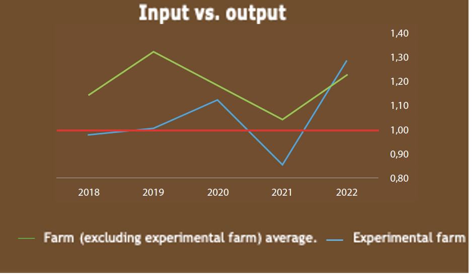
Figure 3: Input (monetary) versus output for the experimental farm in green (top) and the rest of the farm in blue (bottom). The red line is the break-even line at 1. So, for every R1 spent (or invested), the graph indicates how much of that R1 will be received back by the investor. In the above scenario, 2022 was a very favourable year for the farm, while 2021 was particularly challenging. We give credit to Kallie Schoeman who captured the concept of this – it is an extremely valuable way to measure a farm’s performance.
Conclusion
The data obtained indicate that an accurate soil classification map provides the strongest correlation with yield. The physical properties of the soil therefore hold the key as to why a certain area performs well (assuming fertilisation and soil fertility are in place) and others do not.
This is something that has been observed worldwide, based on millions of hectares of harvest data. The physical properties of the soil must be managed and improved where possible (such as compaction, drainage etc.) but generally, drastic change in these properties cannot be achieved. Soil classification remains the most important base map to do variable rate applications.
The physical characteristics, i.e. the true drivers behind production, vary from area to area, and farm to farm, but the answer will always be found in the soil.
